Calculus of
Variations
|
Lecture (starts April 23)
|
| Tuesday |
11:45 - 13:15
|
room 48/582
|
| Thursday |
11:45 - 13:15
|
room 48/582
|
|
Handwritten lecture notes can be found in the library.
Brief Summary:
The purpose of the course is to demonstrate
the beauty and power of variational methods in solving many physical and
geometrical problems. The course will give a self contained introduction
to the basic variational concepts. Here are some keywords: first variation,
Gateaux and Frechet derivatives, fundamental lemma, Euler Lagrange equations,
constrained variational problems, Emmy Noether's theorem, second variation,
convexity, Legendre transformation, Hamiltonian formulation, Hamilton Jacoby
theory, weak lower semicontinuous functionals, existence theorems, regularity
results, and many many examples.
Here is an example from
the theory of capillary surfaces:
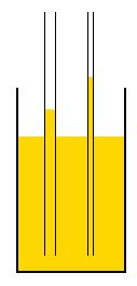 If
you put a transparent straw in a glass filled with orange juice (for example),
you will see that the surface of the orange juice in the straw is a little
bit higher than in the rest of your glass. If you take a straw with a smaller
diameter, the surface is located even higher. What's the reason for that
behavior? The detailed answer will be given in the lecture - but here is
the general recipe. You set up the total energy of the liquid in the straw
consisting of potential energy in the gravitational field and a surface
energy which is proportional to the size of the liquid surface. Writing
things down, you see that the total energy depends on the height function
h(x) which describes the liquid surface. According to a physical principle,
the observed height is the one which minimizes the energy of the system
- that means you have to find the minimum of the energy functional. Taking
the derivative (which is called `variation' in this case) and setting it
to zero, you find a necessary condition for the minimum. This condition
turns out to be a partial differential equation with certain boundary conditions.
Solving it, you can find the minimizer ...
If
you put a transparent straw in a glass filled with orange juice (for example),
you will see that the surface of the orange juice in the straw is a little
bit higher than in the rest of your glass. If you take a straw with a smaller
diameter, the surface is located even higher. What's the reason for that
behavior? The detailed answer will be given in the lecture - but here is
the general recipe. You set up the total energy of the liquid in the straw
consisting of potential energy in the gravitational field and a surface
energy which is proportional to the size of the liquid surface. Writing
things down, you see that the total energy depends on the height function
h(x) which describes the liquid surface. According to a physical principle,
the observed height is the one which minimizes the energy of the system
- that means you have to find the minimum of the energy functional. Taking
the derivative (which is called `variation' in this case) and setting it
to zero, you find a necessary condition for the minimum. This condition
turns out to be a partial differential equation with certain boundary conditions.
Solving it, you can find the minimizer ...
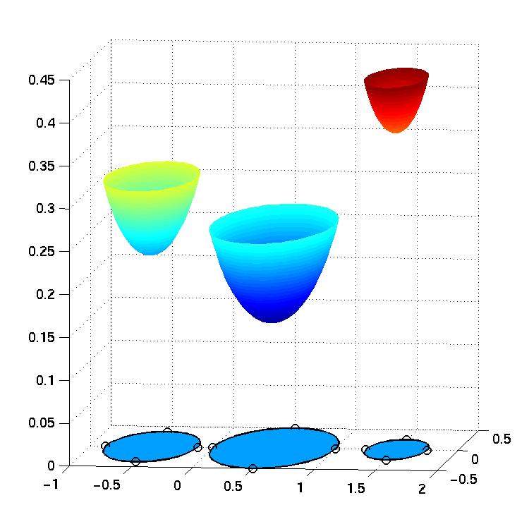
The result of such a calculation can
be seen in the following figure where the capillary surface has been calculated
for three different straw diameters.
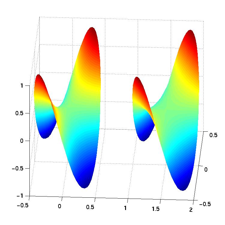
Here is an example from the theory of thin films:
If you take a wire hoop, bend it, and put it into soap liquid, you will
observe a soap film in your wire frame once you remove it from the liquid.
The shape of this surface is dictated again by the principle of least surface
energy (it is surface of minimal area, i.e. a minimal surface).
Going through the same process as described above: setting up the energy
functional, taking its first variation and equating it to zero, you find
a partial differential equation with boundary conditions as necessary condition
for the surface to be minimal. The linearization of this PDE is the good
old Laplace equation. Here is an exemplary solution: the graph on the right
is the minimal surface for the given boundary curve (your wire hoop) and
the graph on the left is the same calculation carried out with the simpler
Laplace equation.
Here is an example from geometrical optics:
According to Fermat's principle, a ray of light travels from a light
source to an observer in such a way that the total travel time is minimized
(the total travel time is a functional which assigns numbers
to curves, i.e. functions - finding the physical ray requires minimization
of the functional). Since the speed of light depends on the refraction
index of the medium, the resulting path need not be a straight line if
the refraction index is space dependent. For example, the density of the
air (and thus also the refraction index) changes with height in the earth's
atmosphere. Optical effects of this variation in the refraction index are
most prominent for light rays which enter the atmosphere close to the horizon:  just
before sunset, the sun appears rather like an ellipse than a circle (flat),
stars close to the horizon appear to be higher in the sky than they should
be and so on...
just
before sunset, the sun appears rather like an ellipse than a circle (flat),
stars close to the horizon appear to be higher in the sky than they should
be and so on...
Using the vanishing first variation as necessary condition for a minimum
of the total time functional, one derives an ordinary differential equation
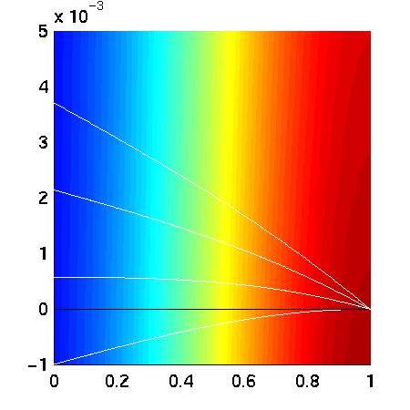
for the light curve. Below, this equation is solved with several Neumann
conditions on the left (prescribing the angle of the entering ray) and
a Dirichlet condition on the right (the eye of the observer). The color
indicates the refraction index which increases from blue to red.
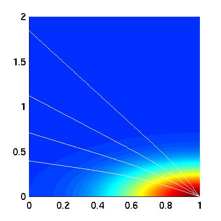
The following example shows the typical form of light rays which enter
the earth's atmosphere almost parallel to the horizon (sun set). The observer
is located at the point (1,0) and the black line indicates the horizon
(= tangent to the observer's position). The density is assumed to be radially
symmetric with respect to the center of the earth. The corresponding refraction
index is color coded in the graph below (blue=vacuum index, red=high index).
One can see that, even if the sun is below the horizon, light rays can
reach the observer's eye.
Since the human brain assumes that light rays are straight lines the observer
thinks that the angular height of a light source over the horizon is equal
to the slope of the ray just before it hits the retina. Notice that this
slope is actually larger than the "true" slope which would be experienced
without a disturbing atmosphere. Consequently, stars close to the horizon
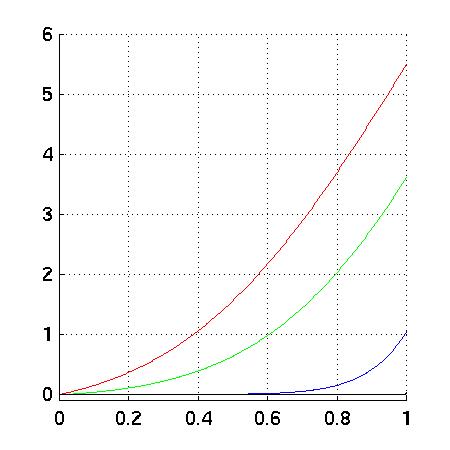
seem to be higher than they really are. The slope discrepancy reduces with
increasing height. To see this more carefully, the change of the slope
of the light rays is plotted below. The black line belongs to a ray which
is almost orthogonal to the horizon and its slope is essentially unchanged.
In contrast to this, a ray running parallel to the horizon suffers an angle
increase of about 5.5 acrimony (red curve). Intermediate incoming angles
(green and blue curves) are increased correspondingly (the higher the less).
Now it is easy to explain the flat sun at sunset: The lower part of
the sun is raised more than the upper part so that it becomes flat (rays
entering at the same height are, of course treated in the same way so that
the width of the sun is unchanged).
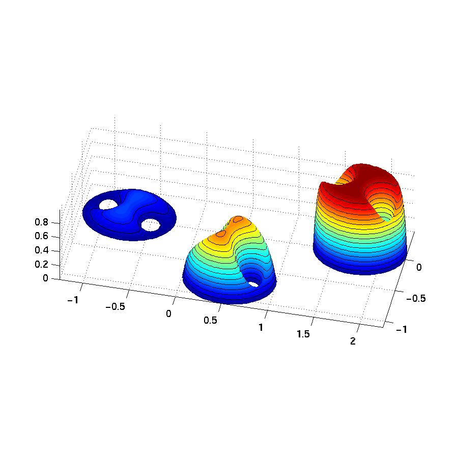
Here is a Hilbert-space example:
What happens if you project the constant one function onto the space
of H1(A) functions which vanish at the
boundary of A? Using the standard H1 scalar
product, you get a function which is far away from the one function in
the "picture norm". However, if you introduce a weight in the scalarproduct
which reduces the importance of the L2
norm of the derivatives the projection shows more resemblance with the
constant one function. Below you see an example where A is an ellipse with
two holes punched into it. The weights in front of the L2
norm of the derivatives are (from left to right) 1/10, 1/100, 1/1000.
In the language of variational calculus: the functional is the square
of the (weighted) H1 distance to the one
function and the necessary condition for a minimum (vanishing first variation)
leads to a Helmholtz equation with unit source.