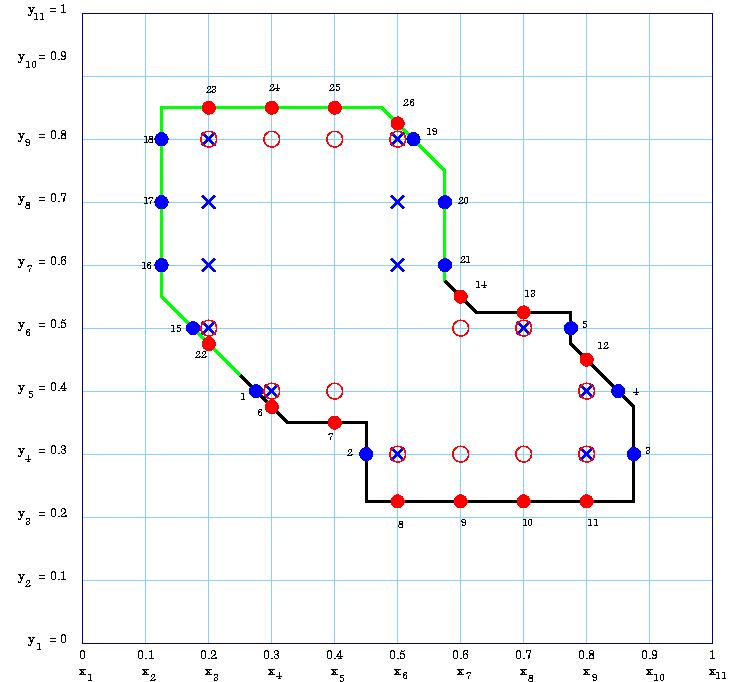
Light blue lines indicate the grid lines and the domain
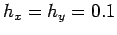
 is in this case a unit square with
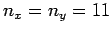 and
and
 . On the black marked
part of the boundary, Dirichlet boundary condition is given,
the green one is the Neumann boundary.
. On the black marked
part of the boundary, Dirichlet boundary condition is given,
the green one is the Neumann boundary.
| Start page of documentation | Download the code | Documentation: PDF, PS |
| Previous: Visualisation of the results | Next: Bibliography |
If you are going to replace the built-in geometry pre-processor by your own one, it has to provide the interface structure IX. Probably the best way to explain how it has to look like is a concrete example.
Light blue lines indicate the grid lines and the domain
is in this case a unit square with
and
. On the black marked
part of the boundary, Dirichlet boundary condition is given,
the green one is the Neumann boundary.
Blue filled circles mark x-type intersection points, red filled circles are intersection points of y-type. Blue crosses mark the anchor points for x-intersections, red empty circles mark the anchor points for y-intersections.
Interface structure has following fields:
 the anchor is defined as follows:
It is a point
the anchor is defined as follows:
It is a point
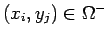 such that
 and
and
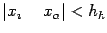
 and
and
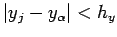
 has to form a right hand system. In two dimensions,
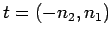 .
.
Ordering of the intersection points
Currently, the code is constructed in such way that IX has to consist of two
parts, IX_D (contains points along the Dirichlet boundary) and IX_N (contains the intersection points along the Neumann boundary).
It is,

Each of structures IX_D and IX_N has to be ordered in such way that x-type intersections come first and then come y-intersections.
In our example this would look as follows:
| Nr | Nr | Nr | |||||
| (IX) | (IX_D) | (IX_N) | coord | type | anch | n | t |
| 1. | 1. | - | 0.275, 0.400 | `x' | 4, 5 | (-1, -1) |
(1, -1) |
| 2. | 2. | - | 0.450, 0.300 | `x' | 6, 4 | (-1, 0) | (0, -1) |
| 3. | 3. | - | 0.875, 0.300 | `x' | 9, 4 | (1, 0) | (0, 1) |
| 4. | 4. | - | 0.850, 0.400 | `x' | 9, 5 | (1, 1) |
(-1, 1) |
| 5. | 5. | - | 0.775, 0.500 | `x' | 8, 6 | (1, 0) | (0, 1) |
| 6. | 6. | - | 0.300, 0.375 | `y' | 4, 5 | (-1, -1) |
(1, -1) |
| 7. | 7. | - | 0.400, 0.350 | `y' | 5, 5 | (0, -1) | (1, 0) |
| 8. | 8. | - | 0.500, 0.225 | `y' | 6, 4 | (0, -1) | (1, 0) |
| 9. | 9. | - | 0.600, 0.225 | `y' | 7, 4 | (0, -1) | (1, 0) |
| 10. | 10. | - | 0.700, 0.225 | `y' | 8, 4 | (0, -1) | (1, 0) |
| 11. | 11. | - | 0.800, 0.225 | `y' | 9, 4 | (0, -1) | (1, 0) |
| 12. | 12. | - | 0.800, 0.450 | `y' | 9, 5 | (1, 1) |
(-1, 1) |
| 13. | 13. | - | 0.700, 0.525 | `y' | 8, 6 | (0, 1) | (-1, 0) |
| 14. | 14. | - | 0.600, 0.550 | `y' | 7, 6 | (1, 1) |
(-1, 1) |
| 15. | - | 1. | 0.175, 0.500 | `x' | 3, 6 | (-1, -1) |
(1, -1) |
| 16. | - | 2. | 0.125, 0.600 | `x' | 3, 7 | (0, -1) | (1, 0) |
| 17. | - | 3. | 0.125, 0.700 | `x' | 3, 8 | (0, -1) | (1, 0) |
| 18. | - | 4. | 0.125, 0.800 | `x' | 3, 9 | (0, -1) | (1, 0) |
| 19. | - | 5. | 0.525, 0.800 | `x' | 6, 9 | (1, 1) |
(-1, 1) |
| 20. | - | 6. | 0.575, 0.700 | `x' | 6, 8 | (1, 0) | (0, 1) |
| 21. | - | 7. | 0.575, 0.600 | `x' | 6, 7 | (1, 0) | (0, 1) |
| 22. | - | 8. | 0.200, 0.475 | `y' | 3, 6 | (-1, -1) |
(1, -1) |
| 23. | - | 9. | 0.200, 0.850 | `y' | 3, 9 | (0, 1) | (-1, 0) |
| 24. | - | 10. | 0.300, 0.850 | `y' | 4, 9 | (0, 1) | (-1, 0) |
| 25. | - | 11. | 0.400, 0.850 | `y' | 5, 9 | (0, 1) | (-1, 0) |
| 26. | - | 12. | 0.500, 0.825 | `y' | 6, 9 | (1, 1) |
(-1, 1) |
| Previous: Visualisation of the results | Next: Bibliography |