| Start page of documentation | Download the code | Documentation: PDF, PS |
| Previous: Correction terms | Next: Solving the resulting system |
At first, jumps are expressed in terms of known quantities, like boundary conditions, and one sided derivatives. Then, for jumps at arbitrary intersection point we can write equations
Note that the one sided derivatives depend on the unknown solution. Our goal is to approximate them using a least squares fit of a quadratic polynomial.
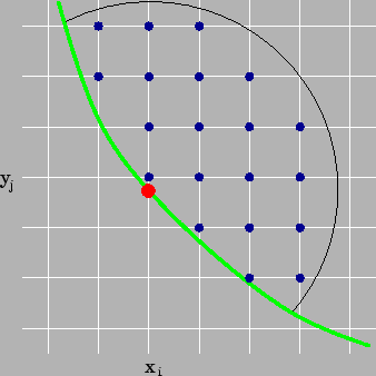
The first step is to select the stencil for least squares interpolation.
We follow the methodology from [3].
It is done by selecting some radius
 and then taking all grid points
of
and then taking all grid points
of  inside circle with radius
 . (Line 73 in
DIFFOP/d_matrix.m.) With
. (Line 73 in
DIFFOP/d_matrix.m.) With  we denote the stencil cardinality.
For each stencil point we try to fit a quadratic polynomial:

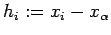 and
and
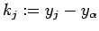 . With this a weighted
least squares problem is obtained:
. With this a weighted
least squares problem is obtained:
![$\displaystyle \sum_{(x_i,y_j)\in\mbox{ stencil}} w_{i,j}^2 \left( p(x_i,y_j) - u_{i,j} \right)^2
\xrightarrow[P]{} \min
$](img97.png)
 . In the code the following
weights are used:
. In the code the following
weights are used:

For a given grid function  , coefficients of the polynomial are
given by
, coefficients of the polynomial are
given by


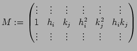
Matrix  is the restriction operator,
  restricts the
vector defined at all grid points to its values only at
the stencil points. is possible to write explicitely, however,
we have found that this costs enormous computational time and
because of this reason in code the matrix
restricts the
vector defined at all grid points to its values only at
the stencil points. is possible to write explicitely, however,
we have found that this costs enormous computational time and
because of this reason in code the matrix  is directly
computed (matrix W2R in DIFFOP/d_matrix.m).
is directly
computed (matrix W2R in DIFFOP/d_matrix.m).
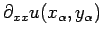
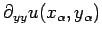
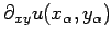
Note that
 |
 |
 |
|
 |
|
 |
|
 |
|
 |
|
 |
|
 |
|
 |
|
 |
|
 |
|
 |


 corresponds the
variable B.
corresponds the
variable B.
Using (8) we obtain in the case of Dirichlet boundary condition
![\begin{displaymath}
\begin{array}{cccccc}
0\cdot B(1,:) &U &+& [u] &=& -u_D \\
...
...mbox{These form vector } \tilde F}{\underbrace{ 0}}
\end{array}\end{displaymath}](img121.png)
Using (9) we get for Neumann boundary
![\begin{displaymath}
\begin{array}{cccccc}
1\cdot B(1,:)& U &+& [u] &=& 0 \\
\le...
...mbox{These form vector } \tilde F}{\underbrace{ 0}}
\end{array}\end{displaymath}](img122.png)
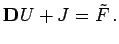
Thus, the system for jumps can be written as
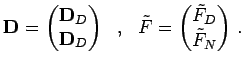
In code, the matrix
 (stored in variable D)
and the right hand side vector
(stored in variable D)
and the right hand side vector  (stored in variable Ft)
consist each of two parts, corresponding to Dirichlet and Neumann
intersection points:
(stored in variable Ft)
consist each of two parts, corresponding to Dirichlet and Neumann
intersection points:
Note: matrix
and vector depend
on boundary conditions!
| Previous: Correction terms | Next: Solving the resulting system |
![\begin{displaymath}\begin{array}{rcccl} && [u] &=& -u_D \partial_x u^- & + & ...
...0 \partial_{xy} u^- & + &[\partial_{xy} u] &=& 0 \end{array}\end{displaymath}](img89.png)
![\begin{displaymath}\begin{array}{rcccl} u^- & + &[u] &=& 0 t_1^2 \partial_x u...
...0 \partial_{xy} u^- & +& [\partial_{xy} u] &=& 0 \end{array}\end{displaymath}](img90.png)