| Start page of documentation | Download the code | Documentation: PDF, PS |
| Previous: Discretisation in a rectangle | Next: Additional equations for jumps |
The points where the 5-point stencil is cut by the interface are called irregular points. There, the approximation (2) has to be corrected by adding so called correction terms. They can be written for each of the appearing derivatives in (1) separately.
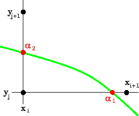
Consider a situation like in figure above and
let
 be the coordinates of the
intersection point
be the coordinates of the
intersection point  and
and
 : coordinates of the
intersection point
: coordinates of the
intersection point  .
Let
.
Let
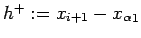 ,
,
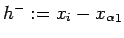 ,
,
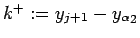 ,
,
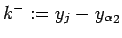 . Then, the
corrected differences of second order derivatives are
. Then, the
corrected differences of second order derivatives are
 -direction and similarly for the
 -derivatives
![$ [u]$](img59.png) ,
,
![$ [\partial_x u]$](img60.png) ,
,
![$ [\partial_y u]$](img61.png) ,
,
![$ [\partial_{xx}u]$](img62.png) ,
,
![$ [\partial_{yy}u]$](img63.png) and
and
![$ [\partial_{xy}]$](img64.png) , where in the case of
Poisson equation some of them are redundant.
, where in the case of
Poisson equation some of them are redundant.
In general, jump in
the mixed derivative is not used in expressions
(3-6) and
jumps in -derivatives are not used at
-intersections, as well as
jumps in -derivatives are not used in -intersections.
All jumps are stored in one supervector  (see
ASSEMBLE/run_ejiim.m, variable J) with ordering
(see
ASSEMBLE/run_ejiim.m, variable J) with ordering
![$\displaystyle J = ([u]_{\alpha_1}, [\partial_x u]_{\alpha_1}, [\partial_{y} u...
...al_{xy}u]_{\alpha_1},
[u]_{\alpha_2}, \ldots, [\partial_{xy}u]_{\alpha_l})
$](img66.png)
 is the number of intersection points , , ...,
 . Coefficients of in the correction terms
(3-6) are stored in matrix
. Coefficients of in the correction terms
(3-6) are stored in matrix
 , in code denoted by P (see ASSEMBLE/run_ejiim.m).
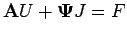
With this, approximation of the differential operator
 in domain
  can be written as
Matrix
, in code stored in variable P is constructed
of two parts
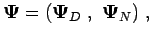
 corresponds to intersection points belonging to
 and
and
 - to intersection points along
 .
.
Each of
and
is constructed as
sum
 |
 |
 |
|
 |
|
 |
 corrects the approximation of
 derivative according to (3,4) and
 corrects the approximation of
 derivative according to (5,6).
See ASSEMBLE/run_ejiim.m.
derivative according to (5,6).
See ASSEMBLE/run_ejiim.m.
Note: Matrix  depends only on the differential operator and
geometry. No dependence on boundary conditions!
depends only on the differential operator and
geometry. No dependence on boundary conditions!
Construction of the matrix
is done in function
DIFFOP/corrections.m.
The interface information is stored in the structure variable IX, see
Section 3 for details.
Constructing of
matrix
Idea: run a loop over all intersection points and check, which grid points are affected.
We know that
derivative is affected only
by -type intersections, so the matrix
has zeros in the right block, corresponding to -type
intersection points.
In a loop over all -intersections:
 .
.
Construction of
is done completely analogously,
only now zeros are in the left block of
and loop
has to be done over all intersections.
In the actual version of the code, the EJIIM system is solved
by Matlab `
 '-operator. For larger problems, especially
three dimensional, the Schur-complement approach together with
some fast solver for inverting the operator
'-operator. For larger problems, especially
three dimensional, the Schur-complement approach together with
some fast solver for inverting the operator
 is highly
suggested [3,1,2].
is highly
suggested [3,1,2].
| Previous: Discretisation in a rectangle | Next: Additional equations for jumps |


![$\displaystyle \frac{1}{h_x^2}\left(u_{i+1,j}-2u_{i,j}+u_{i-1,j}\right)
-\frac{1...
...partial_x u]_{\alpha_1}
+ \frac{1}{2}(h^+)^2 [\partial_{xx}u]_{\alpha_1}\right)$](img52.png)
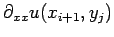
![$\displaystyle \frac{1}{h_x^2}\left(u_{i+2,j}-2u_{i+1,j}+u_{i,j}\right)
+\frac{1...
...partial_x u]_{\alpha_1}
+ \frac{1}{2}(h^-)^2 [\partial_{xx}u]_{\alpha_1}\right)$](img54.png)

![$\displaystyle \frac{1}{h_y^2}\left(u_{i,j+1}-2u_{i,j}+u_{i,j-1}\right)
-\frac{1...
...partial_y u]_{\alpha_2}
+ \frac{1}{2}(k^+)^2 [\partial_{yy}u]_{\alpha_2}\right)$](img56.png)
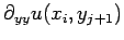
![$\displaystyle \frac{1}{h_y^2}\left(u_{i,j+2}-2u_{i,j+1}+u_{i,j}\right)
+\frac{1...
...partial_y u]_{\alpha_2}
+ \frac{1}{2}(k^-)^2 [\partial_{yy}u]_{\alpha_2}\right)$](img58.png)
 and (
and ( .
.
